The Iris dataset was made famous by British statistician/biologist Ronald Fisher in 1936, and has been widely used in the statistical pattern recognition literature ever since. The dataset consists of 150 instances, with 50 belonging to each of three species of Iris – Setosa, Virginica and Versicolor. The objective is to predict the species an instance belongs to based on the values of four continuous features: the length and width of sepals, and the length and width of petals.
Generating Synthetic Examples
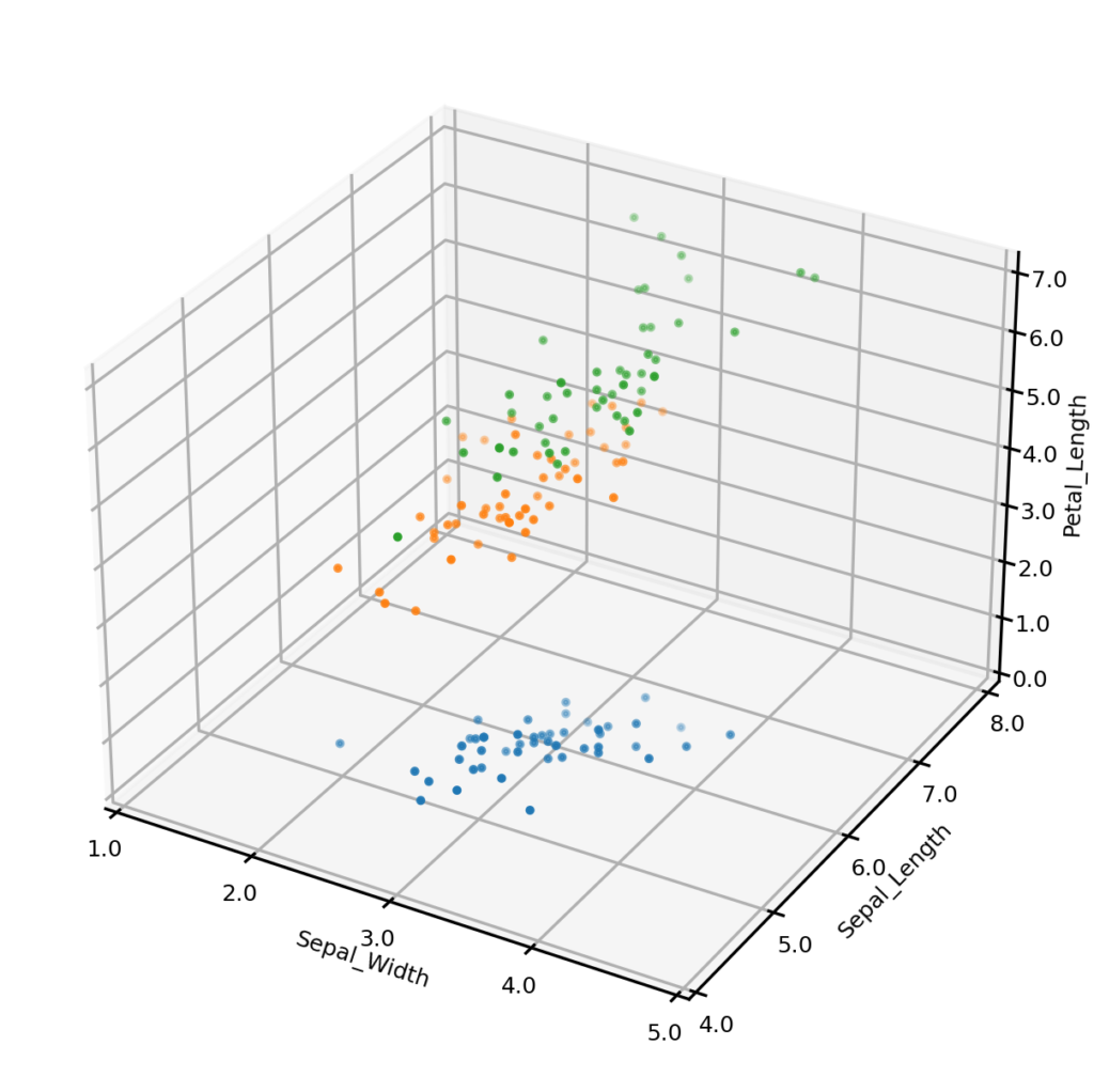
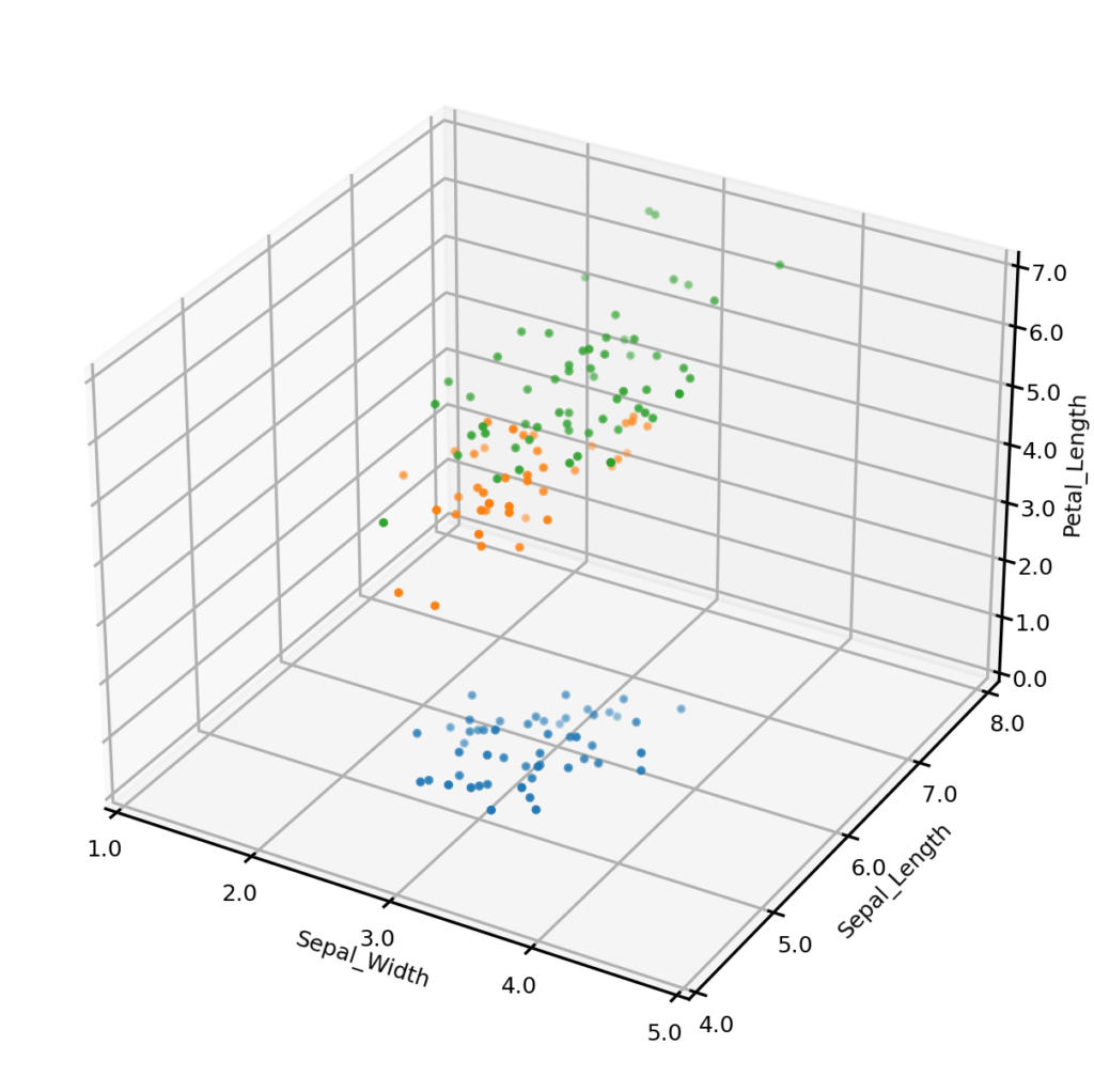
The UNCRi synthetic data generator was used to generate 150 synthetic data points for the Iris dataset. The plots below show the original dataset (left) and a synthetic dataset (right), with three of the four continuous variables plotted along the axes, and species represented by color. It is clear from visual inspection that the synthetic examples follow the same general distribution as the originals. (We demonstrate how we can test claim more formally in another blog).
Iris dataset - original examples
Iris dataset - synthetic examples
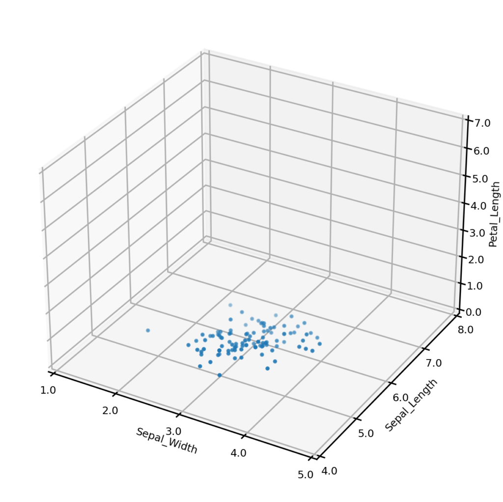
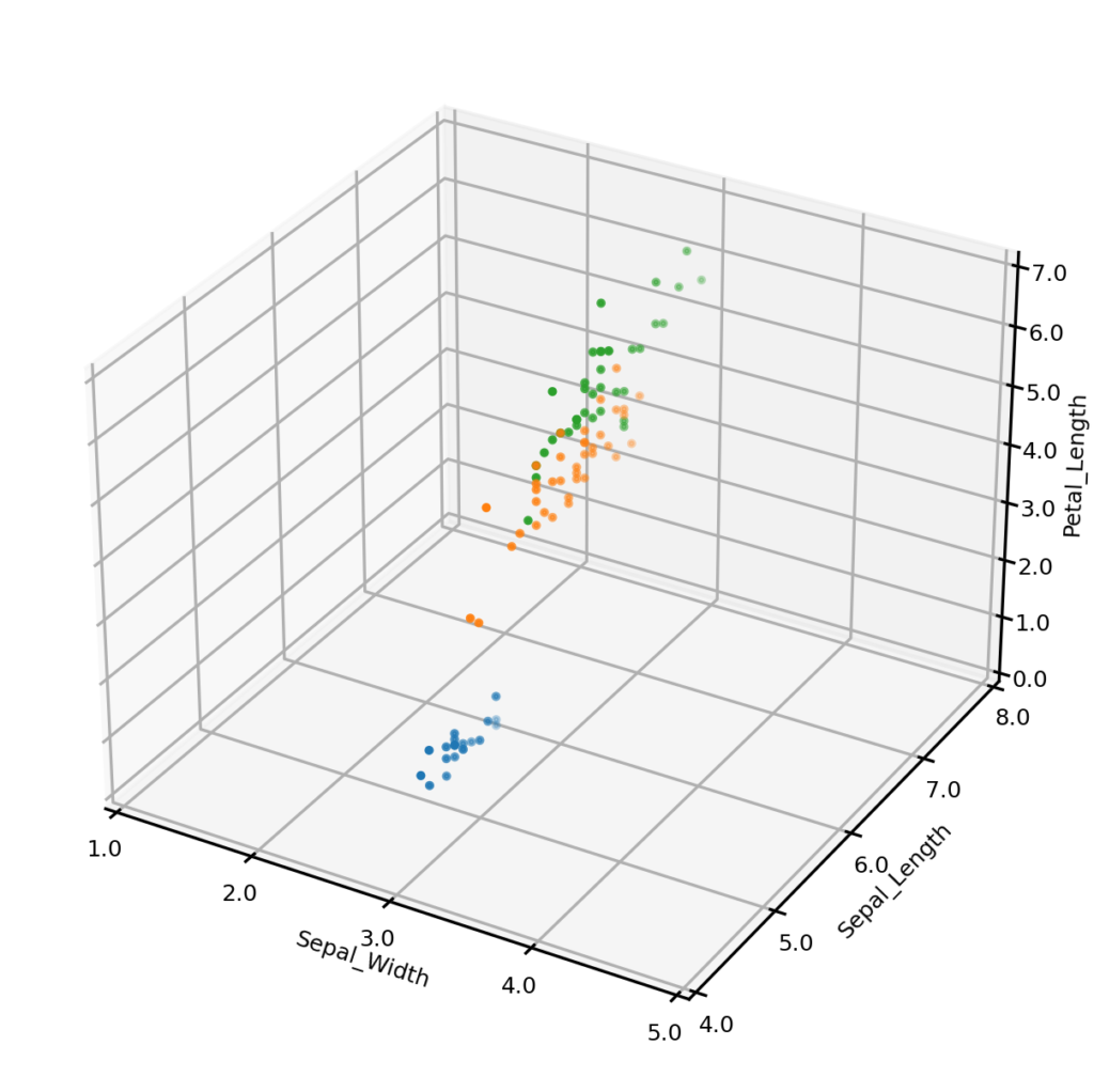
It is also possible to generate synthetic data matching one more conditions on multiple variables. For example, we may wish to only generate synthetic examples from one class – the plot below left shows synthetic examples conditional on class being Iris-setosa. Or we may wish to impose some condition on the values that one or more numerical variables may take – the plot below right shows synthetic examples conditional on Sepal_width having a value of exactly 3.0. We could also impose both of these conditions simultaneously (not shown). Importantly, UNCRi does not simply generate examples from the unconditional distribution and then filter those matching the condition (which would be extremely efficient under the condition that a continuous variable take an exact value). The examples are generated from the estimated conditional distributions. This makes the UNCRi approach highly efficient in situations where the conditions occur rarely in the original dataset.
Synthetic examples conditional on Species = 'Iris-setosa'
Synthetic examples conditional on Sepal_width=3.0
Estimating the Joint Probabilities
Except for the case of uniform distributions (where all datapoints are equally likely to occur), some data points are likely to occur more frequently than others. For example, for a one-dimensional normally distributed variable, values close to the mean are more likely to be observed than values in the tails. The UNCRi framework allows us to estimate these ‘joint distributions’ on complex, high dimensional datasets.
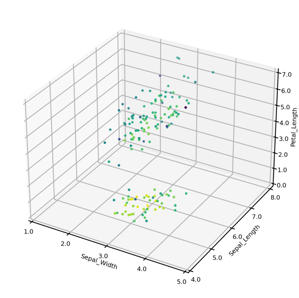
The plot below shows the estimated joint probabilities for both the original Iris dataset (left) and synthetic dataset (right), where the color of points indicates the joint probability, with the blue end of the spectrum representing low probability and the yellow representing high probability. From visual inspection we can see that the joint probabilities display the same general distribution in each case.
Original examples (color indicates joint probability)
We can also compare the one-dimensional distribution of joint probabilities. The histograms below shows the distribution of probabilities for the original examples (left) and synthetic examples (right). (Actually we compare the negative logarithm of the joint probability, but this is unimportant to the following discussion). The distributions have similar means, and each has maximum values of approximately 7.5, but the synthetic data clearly contains some data points which are less likely than those in the original dataset. This is a pattern that we observe for many datasets. While this can be partially explained by the fact that we are estimating the variance of the population from a small sample, there are probably other factors at play. For example it may be the case that the original sample of 150 examples simply did not contain any of these low probability examples, or perhaps they were rejected from some reason.
Distribution of probabilities on original examples
Distribution of probabilities on synthetic examples
The ‘Average Maximum Similarity’ test
In any exercise where synthetic examples are generated, it is important to test whether the synthetic examples are too similar to the original examples. That is, are we simply generating data points which are slightly perturbed versions of the original data points? A simple test for this is what we refer to as the ‘Average Maximum Similarity’ test (or equivalently the ‘Average Minimum Distance test). The test works as follows.
For the original dataset calculate the average similarity between each datapoint and its closest neighbor and call this O_max. For the synthetic dataset find the similarity between each point and its closest neighbor in the ‘original’ dataset and call this S_max. Compare O_max and S_max. If S_max is less than O_max, this indicates that the synthetic examples are probably too close to the original examples. Ideally O_max and S_max should be roughly equal, but in practice we often find that S_Max is slightly greater, which is consistent with what we observed above when comparing the histograms showing the distributions of joint probabilities. (Note that when using the Maximum Average Similarity test it is important that the number of datapoints in the synthetic dataset is the same as that in the original dataset).
Applying the Average Maximum Similarity test to the Iris data resulted in an O_max value of 94.9% and an S_max value of 94.1%, indicating that the generated examples are no closer on average to the original samples than the original samples are to each other. In practice, we have not come across a single instance in which a dataset synthetically generated by the UNCRi framework has failed the maximum average similarity test. This is because the UNCRi framework generates synthetic examples by sequential imputation; i.e., it estimates the distribution of a variable conditional on the values of all variables which have already had a value imputed, and then draws a value from this distribution. The hyperparameters which control the estimate of the conditional distributions have been optimized using a validation procedure which guards against the possibility of these conditional distributions being overfitted.
Key take-aways
The UNCRi framework can be used to generate synthetic examples drawn from the same distribution as the original examples; it can also efficiently generate examples matching some condition.
The UNCRi framework can also estimate the joint probabilities, allowing us to identify potential outliers.
The ‘Maximum Average Similarity’ test can be used to guard against the possibility that generated examples are too close to the originals.