The Iris dataset was made famous by British statistician/biologist Ronald Fisher in 1936, and has been widely used in the statistical pattern recognition literature ever since. The dataset consists of 150 instances, with 50 belonging to each of three species of Iris – Setosa, Virginica and Versicolor. It has traditionally been used in classification tasks where the objective is to predict the species based on the values of four continuous features: the length and width of sepals, and the length and width of petals. We include it as a case study because its low dimensionality makes it easy to visualize, allowing us to get a ‘feel’ for the tasks that can be performed using the UNCRi framework.
Generating Synthetic Examples
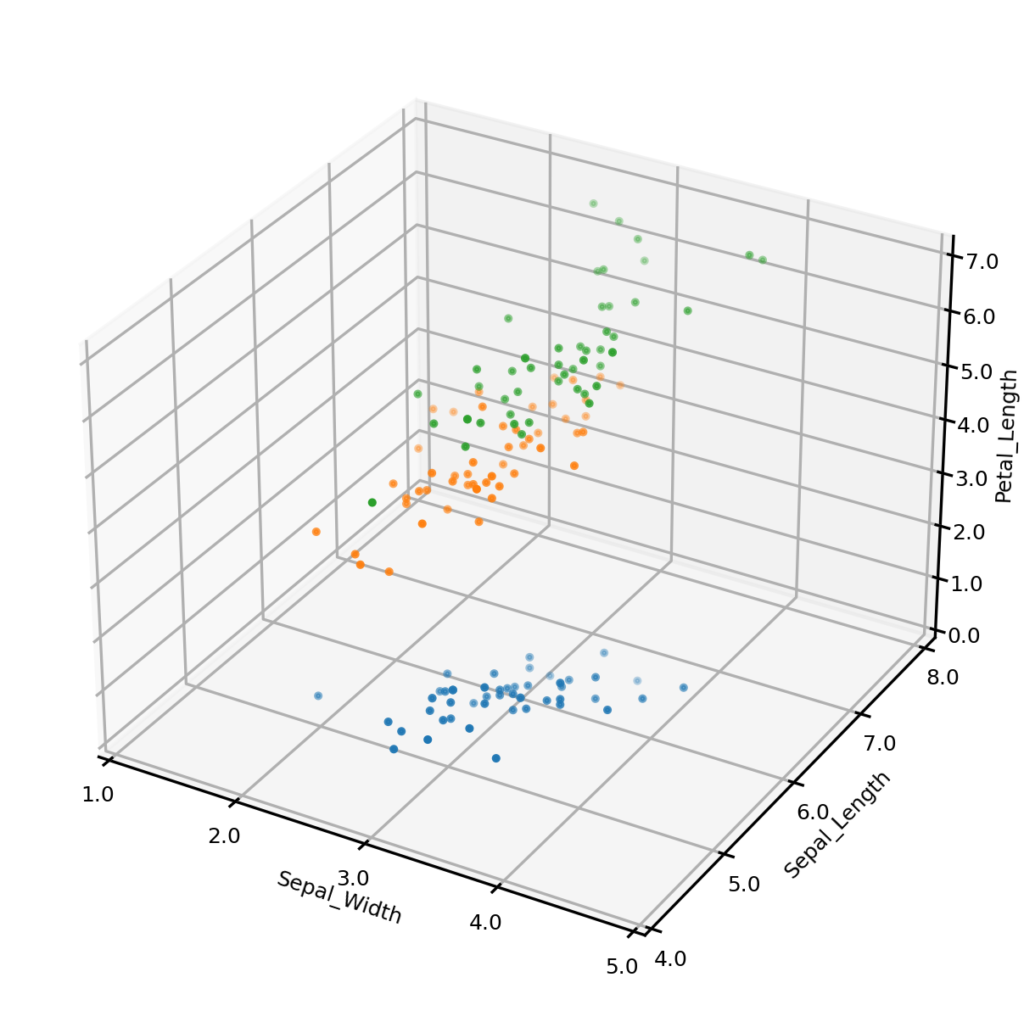
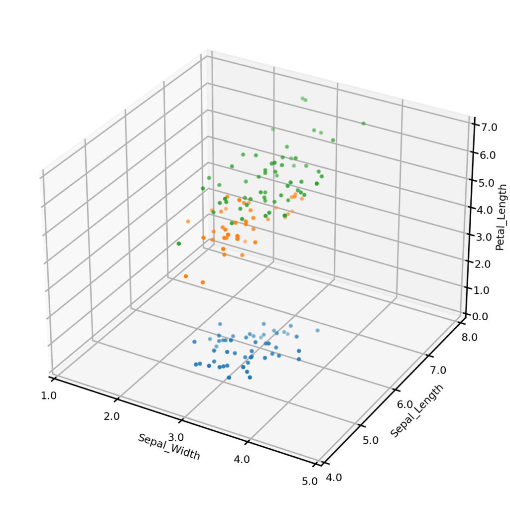
Let’s begin by generating some synthetic data. To do this, we first create an UNCRi model, and then use it to generate 150 synthetic data points. The plots below show the original dataset (left) and the synthetic dataset (right), with three of the four continuous variables plotted along the axes, and species represented by color. It is clear from visual inspection that the synthetic examples follow the same general distribution as the originals. On a more complex dataset, we might also compare univariate and bivariate distributions, but we won’t do so on this case.
Iris dataset - original examples
Iris dataset - synthetic examples
Conditional Synthetic Data
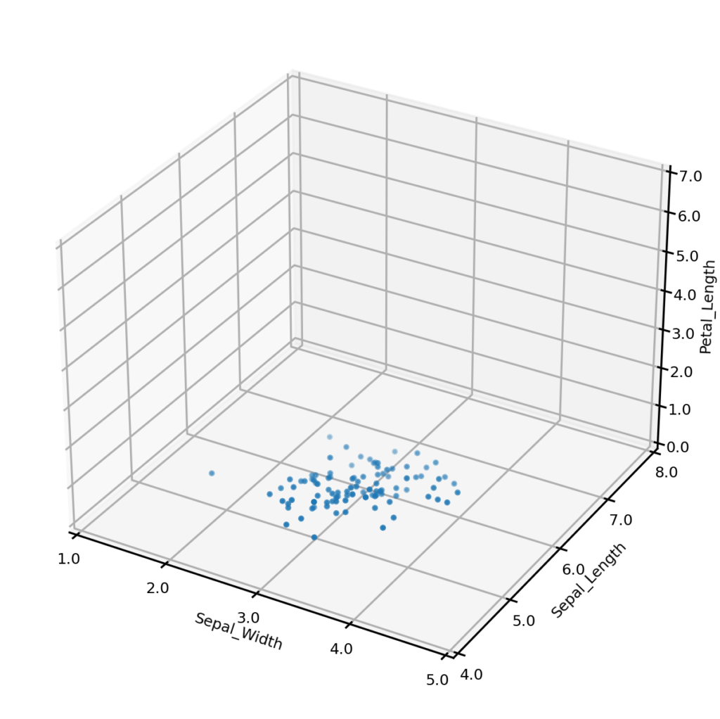
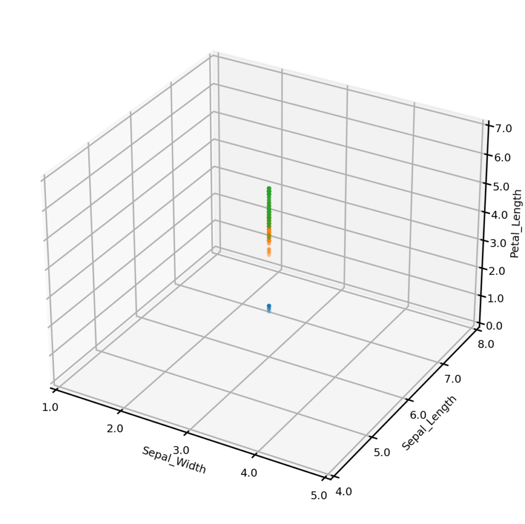
In some cases we may wish to generate conditional synthetic data; i.e., synthetic data matching one more conditions. For example, we may wish to only generate synthetic examples from one class (perhaps to address a class imbalance). The plot below left shows synthetic examples conditional on class being Iris-setosa. Or we may wish to impose some condition on the values that one or more numerical variables may take. The plot below center shows synthetic examples conditional on Sepal_width having a value of exactly 3.0, and the plot below right shows examples having Sepal_width 3.0 AND Sepal_length 6.0.
Synthetic examples conditional on Species = 'Iris-setosa'
Synthetic examples conditional on Sepal_width=3.0
Synthetic examples conditional on Sepal_width=3.0 and Sepal_Length=6.0
Importantly, UNCRi does not simply generate examples from the unconditional distribution and then filter those matching the condition (which would be extremely inefficient under the condition that a continuous variable take an exact value). Under the UNCRi framework the examples are generated directly from the estimated conditional distribution. This makes the UNCRi approach highly efficient in situations where the conditions occur rarely in the original dataset. The figure below shows a screenshot of the UNCRi toolbox interface for selecting conditions. Conditionas on catagorical attributes Categorical attributes
Estimating Joint Probabilities
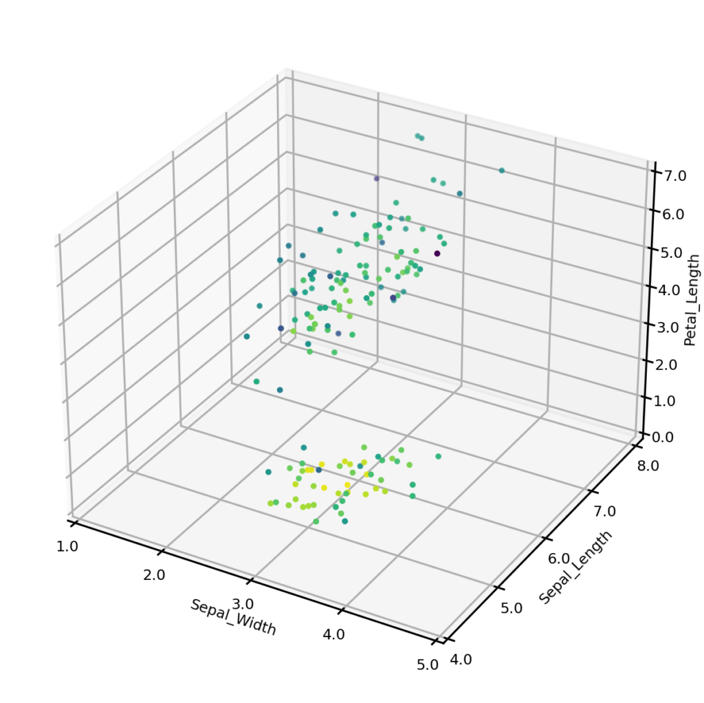
Except for the case of uniform distributions (where all datapoints are equally likely to occur), some data points are likely to occur more frequently than others. For example, for a one-dimensional normally distributed variable, values close to the mean are more likely to be observed than values in the tails. The UNCRi framework allows us to estimate these ‘joint distributions’ on complex, high dimensional datasets. The plot below shows the estimated joint probabilities for both the original Iris dataset (left) and synthetic dataset (right), where the color of points indicates the joint probability, with the blue end of the spectrum representing low probability and the yellow representing high probability. From visual inspection we can see that the joint probabilities display the same general distribution in each case.
Original examples (color indicates joint probability)
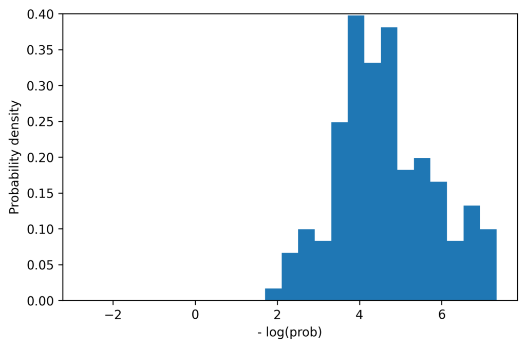
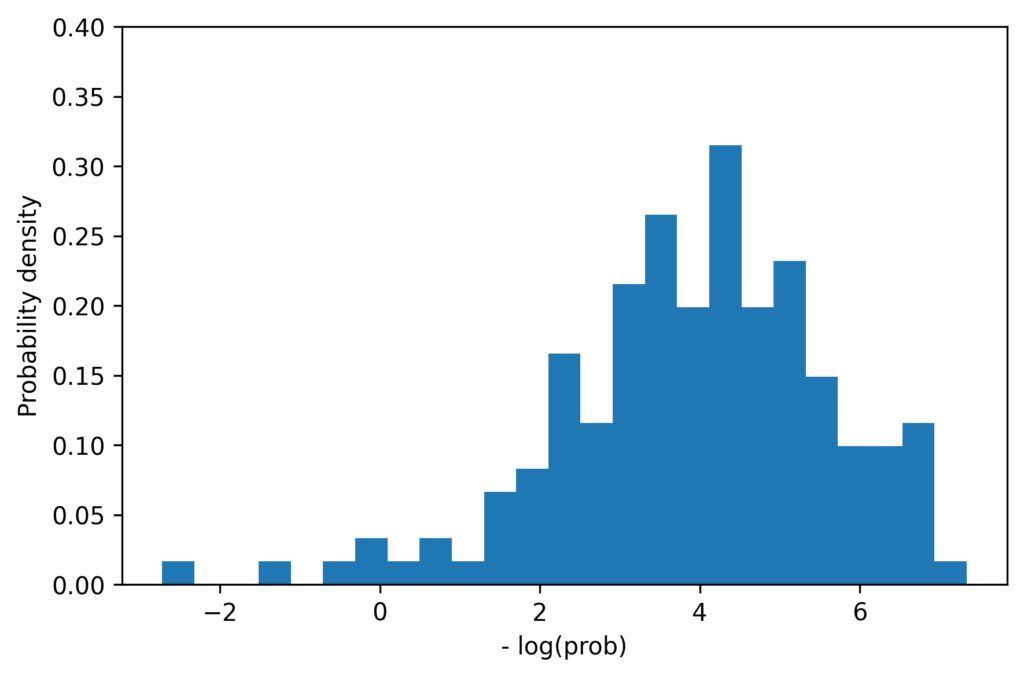
We can also compare the one-dimensional distribution of joint probabilities. The histograms below shows the distribution of probabilities for the original examples (left) and synthetic examples (right). (Actually we compare the negative logarithm of the joint probability, but this is unimportant to the following discussion). The distributions have similar means, and each has maximum values of approximately 7.5, but the synthetic data clearly contains some data points which are less likely than those in the original dataset. This is a pattern that we observe for many datasets. While this can be partially explained by the fact that we are estimating the variance of the population from a small sample, there are probably other factors at play. For example it may be the case that the original sample of 150 examples simply did not contain any of these low probability examples, or perhaps they were rejected from some reason.
Distribution of probabilities on original examples
Distribution of probabilities on synthetic examples
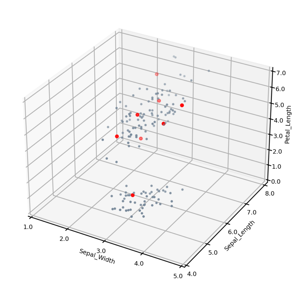
The figure below shows the synthetic data, with the eight lowest probability examples shown in red. Most of them appear towards the outer regions of the two clusters. The one at the bottom of the figure appears not to be an outlier, but this is because one of the variables — Petal-width — is not shown.
Synthetic data points with potential outliers shown in red
The Maximum Similarity test
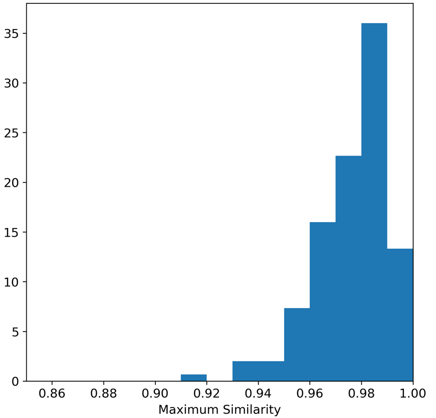
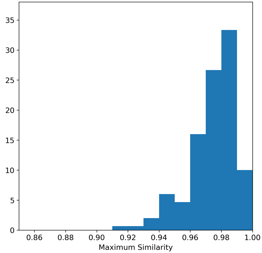
The Maximum Similarity test can be used to determine whether the examples in the synthetic dataset are ‘too close’ to the real examples (see Census Income Case Study for a description). The average maximum similarity between each synthetic example and its closest real example is 0.975, and the average maximum similarity between each real example and its closest real example is 0.977, indicating that the synthetic examples are no closer on average to the real examples than the real examples are to each other. We can also plot histograms to show the distributions of these maximum similarities. The histogram on the left shows the distribution of max similarities between synthetic and real examples, and the histogram on the right shows the distribution of maximum similarities between real examples. Interestingly, in both cases there were instances of the maximum similarity being 1.0. Closer inspection of the iris dataset shows that there in fact two examples in the Iris dataset that are duplicated.
Maximum distances between real examples
Maximum distances between real and synthetic examples
Conclusions
The UNCRi framework was used to create a model for the Iris dataset. The model was then used to generate synthetic examples which had similar distributional characteristics to the originals. Conditional synthetic examples were also generated. Joint probabilities were estimated in order to identify potential outliers. The maximum similarity test was used to identify whether there was any ‘leakage’ of the real examples.