This case study demonstrates how the Skanalytix financial modeling platform generates synthetic financial time series that replicate key statistical and temporal features observed in real markets. These simulations are powered by our proprietary Unified Numeric/Categorical Representation and Inference (UNCRi) framework — the engine behind the platform’s ability to capture complex behaviors without rigid assumptions.
We start with the S&P 500 Index — a cornerstone of global equity markets — then extend the analysis to a portfolio of major technology stocks. The simulated returns serve as the foundation for the scenario-based Value at Risk (VaR) forecasting explored in the next case study. These examples highlight the model’s ability to reproduce stylized facts such as fat tails, volatility clustering, and evolving asset correlations, showcasing its flexibility across both single- and multi-asset applications.
Why Synthetic Market Data Matters
Real-world market data is inherently unpredictable but often lacks sufficient examples of the most consequential scenarios. Rare but critical events like crashes, regime shifts, or extended stress periods are underrepresented in historical datasets. In a rapidly changing world, relying solely on history can leave significant blind spots.
Synthetic data addresses this gap by generating new time series that realistically mimic financial behavior — including downturns, recoveries, and regime transitions — thereby expanding the testing ground for robust financial models. The Skanalytix modeling and simulation platform is designed to fill these gaps with rich, scenario-driven simulations.
However, creating convincing synthetic financial time series is challenging. Markets are noisy, highly interdependent, and governed by complex, non-stationary dynamics. They exhibit well-documented “stylized facts” such as:
Fat tails – Extreme price swings occur more frequently than predicted by a normal distribution.
Volatility clustering – Periods of high and low volatility tend to group together over time.
Mean reversion – Sharp deviations often give way to corrective movements.
Capturing these features accurately while retaining flexibility to explore hypothetical futures is central to meaningful simulation — and a defining capability of the Skanalytix platform.
Simulating a Market Benchmark: S&P 500 Index
We begin by simulating the S&P 500 Index to demonstrate the framework’s ability to capture key statistical and temporal characteristics from real-world data. Historical prices from January 1, 2010 to January 1, 2020 serve as the training window.
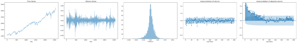
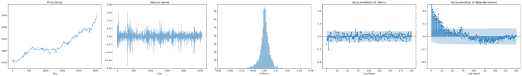
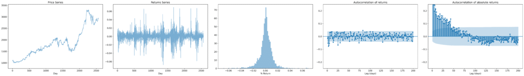
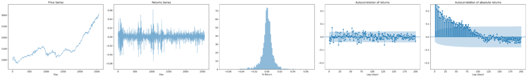
The charts below compare historical data (top row) with synthetic time series generated by the model (second to fourth rows). Each column highlights a key statistical property of the data:
Index level: shows the trajectory of the index over time, capturing long-term trends and the tendency to revert to a moving baseline — a form of mean-reverting behavior typical of aggregate market indices.
Daily returns: illustrates volatility clustering, where periods of high volatility tend to follow each other.
Return distribution: highlights heavy tails, reflecting the higher likelihood of extreme returns compared to a normal distribution.
Autocorrelation of returns: generally close to zero, consistent with the weak-form efficiency of financial markets.
Autocorrelation of absolute returns: demonstrates long memory in volatility, a hallmark of financial time series.
Historical series
Synthetic series
Figure 1. Comparison of historical and synthetic index levels for the S&P 500 index from Jan 2010 to Jan 2020. The synthetic trajectories closely mimic real-world price dynamics, including relative positioning, trend structure, and overall volatility.
The visual comparisons show that the synthetic series closely replicate the historical data — not just in the distribution of returns, but also in the volatility patterns and overall trajectory of the index. This alignment reflects the model’s ability to learn and reproduce the nuanced statistical features of a real financial time series.
Note that the synthetic series were matched in length to the historical data to allow for clear visual comparisons — especially of temporal patterns like volatility clustering and trend behavior. In practice, the Skanalytix platform can generate synthetic data of any desired length.
Visualizing the Return Structure
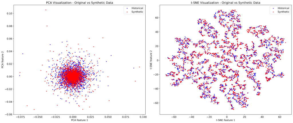
To further assess the realism of the synthetic returns, we apply dimensionality reduction techniques — Principal Component Analysis (PCA) and t-distributed Stochastic Neighbor Embedding (t-SNE) — to both historical and synthetic return series. These methods project high-dimensional return data into two dimensions, making it easier to compare their structural patterns.
Figure 2. PCA and t-SNE visualizations of historic and synthetic returns.
In both cases, points from the synthetic and historical datasets are closely intermingled — a strong visual indication that the synthetic returns share the same underlying structure as the real data. These projections provide intuitive evidence that the model captures the key patterns and relationships that shape financial return behavior.
Simulating Multiple Correlated Assets
Many applications — portfolio construction, risk management, and systemic stress testing — require modeling multiple financial assets simultaneously. Beyond individual return dynamics, multi-asset simulation must capture dependencies shaped by sector linkages, macroeconomic factors, and investor sentiment. These dependencies are dynamic, with correlations often strengthening sharply during stress periods.
Simulating assets independently ignores these important structural connections, leading to unrealistic portfolio behavior. The Skanalytix platform overcomes this by modeling multiple return series jointly, preserving both individual asset characteristics and the dynamic relationships between assets. Key features include:
Cross-asset volatility synchronization
Regime-dependent correlation structures
Consistent return distributions and tail behavior across series
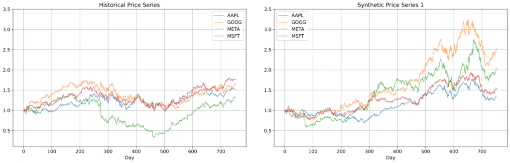
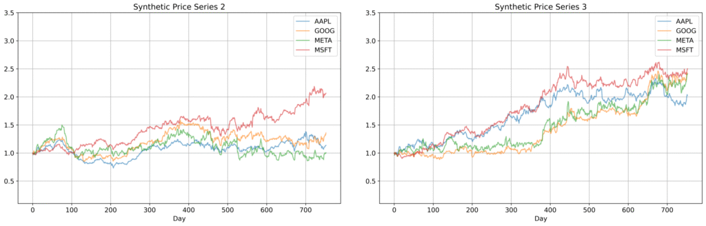
Multi-Asset Example: Major U.S. Technology Stocks
To illustrate, the figures below compare historical and synthetic price series for four major tech stocks — Apple (AAPL), Google (GOOG), Meta (META), and Microsoft (MSFT) — over the period from June 1, 2021 to January 1, 2024. This corresponds to roughly 800 trading days of historical data — a relatively small dataset by typical modeling standards. While this group of tech stocks is not a diversified portfolio, it highlights closely linked behaviors that the Skanalytix framework captures effectively. Its memory-based, nonparametric design (i.e., no fixed functional form, no trained weights) preserves complex dependencies and stylized facts even with limited data — unlike deep generative models, which are technically parametric despite their flexibility. While this example focuses on four assets for clarity, the same framework extends naturally to larger portfolios with many assets and more complex dependency structures.
Figure 3: Comparison of historical and synthetic price trajectories for Apple, Google, Meta, and Microsoft. The synthetic trajectories closely replicate the behavior of each asset while preserving joint dynamics, including synchronized trends and relative movements across stocks.
Comparisons of historical and synthetic price trajectories show that the synthetic assets replicate individual behaviors and joint dynamics, including synchronized trends and relative movements. The synthetic series also exhibit volatility clustering and fat tails, consistent with earlier observations for the S&P 500 (not shown here for brevity).
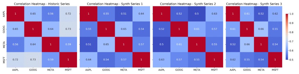
Cross-Asset Correlations
In multi-asset simulations, capturing the structure of return correlations is as important as modeling individual asset behavior. Preserving these relationships enables synthetic data to support realistic stress testing, risk aggregation, and strategy development.
The heatmaps below compare the historical correlation matrix with those from three independently generated synthetic datasets.
Figure 3. Stacked return plots for the four tech stocks showing periods of elevated volatility.
The synthetic series replicate individual asset dynamics and joint episodes of heightened volatility, while the heatmaps confirm that the synthetic data accurately capture both the strength and pattern of cross-asset correlations — all essential for credible multi-asset modeling. Note, however, that these are ‘average’ correlations. As in real financial series, these correlations can change over time — a phenomenon that the Skanalytix platform is designed to capture.
Aligned Volatility Across Assets
A defining feature of systemic market behavior is that volatility doesn’t just cluster within assets — it often aligns across assets. Market-wide stress events, earnings cycles, or macroeconomic shocks can drive multiple assets into periods of heightened or subdued volatility simultaneously.
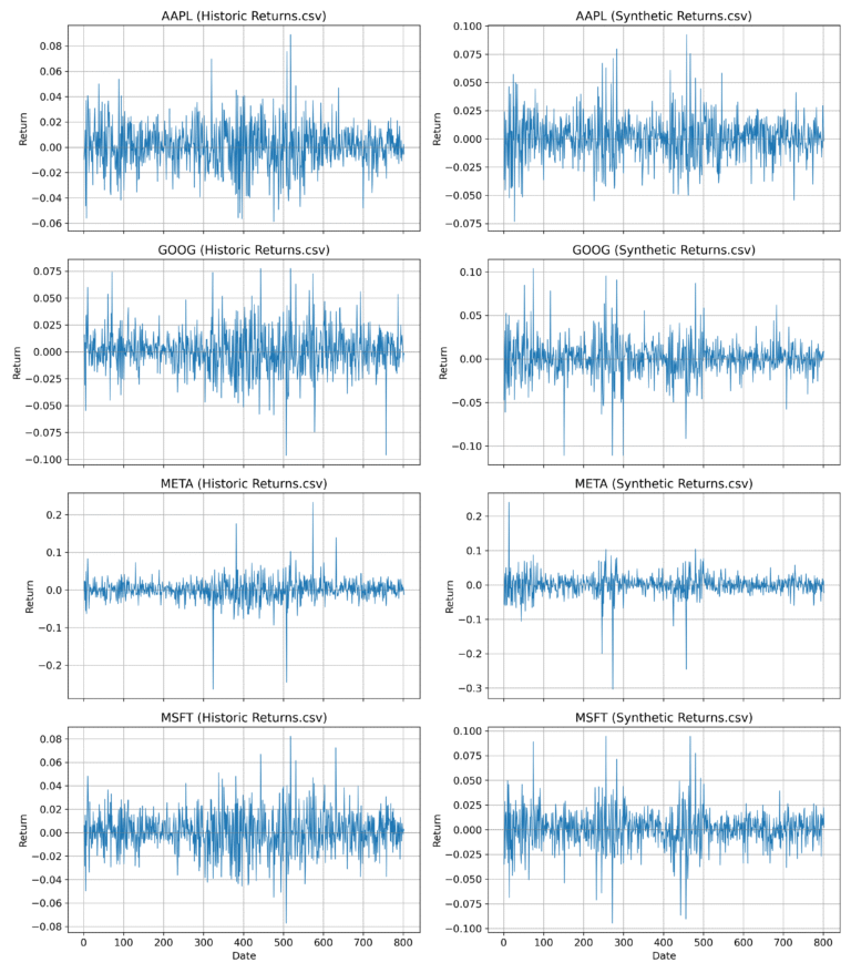
To assess whether our simulations capture this effect, the figure below shows stacked return series for Apple, Google, Meta, and Microsoft. The left panel shows historical returns; the right panel shows a synthetic sample generated by our model.
Figure 4. Stacked daily return series for four major tech stocks — Apple, Google, Meta, and Microsoft. The left panel shows historical data (June 2021–January 2024); the right panel shows synthetic returns. The model captures both individual asset dynamics and joint volatility regimes, with periods of synchronized turbulence clearly visible in both datasets.
Visual inspection reveals strong similarity in volatility alignment across both datasets. In both cases, we observe multi-asset periods of calm punctuated by episodes of synchronized turbulence. These stocks tend to experience large losses simultaneously, creating pronounced tail risk — a feature many conventional risk models fail to capture but which Skanalytix naturally models. This alignment is not imposed; it emerges from the underlying structure of the Skanalytix platform, specifically the UNCRi framework’s ability to learn and replicate joint temporal dynamics across return series.
Looking Ahead: From Simulation to Risk Forecasting
This case study focused on generating realistic synthetic price and return series. Building on this foundation, the next use case — Scenario-Aware Risk Forecasting with Generative Financial Models — uses the same set of four tech stocks to explore scenario-driven risk forecasting. By leveraging the synthetic data produced by the Skanalytix platform — which captures complex joint behaviors and tail risks — we demonstrate how Value at Risk (VaR) and related measures can be estimated more robustly, even in situations where traditional models struggle.
Summary and Outlook
Financial time series exhibit complex stylized behaviors requiring models that capture conditional distributions and temporal dynamics.
The Skanalytix platform is purpose-built to model these complexities, generating synthetic series that replicate key statistical properties while preserving underlying market dynamics. It naturally extends to multi-asset settings, producing realistic correlations, joint behaviors, and synchronized volatility regimes without sacrificing the fidelity of individual assets.
Importantly, this realism is achieved even with relatively small historical datasets — for example, the tech stocks simulation used just over 800 trading days, a volume often insufficient for many deep generative models. The UNCRi framework’s nonparametric, memory-based approach excels in such data-constrained environments.