Overview

The Income dataset (also known as the Adult dataset) is a widely used benchmark for predicting whether an individual earns more than $50K annually based on demographic and employment attributes. This use case demonstrates how the UNCRi framework effectively models mixed-type tabular data without temporal dependencies. We show how UNCRi generates realistic synthetic data, captures complex conditional relationships, and supports predictive tasks despite missing values. Through comprehensive validation — including distribution comparisons, Train-on-Synthetic-Test-on-Real (TSTR) evaluation, joint probability estimation, and privacy-preserving similarity testing — we confirm that UNCRi accurately represents the original data’s statistical structure while preserving privacy. This establishes confidence in applying UNCRi to diverse real-world inference and data augmentation challenges.

The Income Dataset

The Income dataset contains 32,561 instances described by 15 attributes — nine categorical and six numerical. The goal is to classify the binary income attribute (≤50K or >50K) based on the other features. The dataset includes missing values and is not time-series in nature, making it ideal for demonstrating UNCRi’s capabilities on mixed-type tabular data.

Below are excerpts from the original dataset alongside synthetic examples generated by UNCRi. At first glance, the synthetic data appears plausible, but rigorous testing is needed to confirm the model’s accuracy in capturing conditional relationships.

Figure 1: Subset of examples from original dataset (above) and synthetic dataset (below)

As is always the case when using the UNCRi framework, the first step is to create an UNCRi model for the dataset of interest. This model can then be used to perform a variety of tasks. But the tasks can only be performed accurately if the model adequately represents the original data. While visual inspection of the tables above suggest that the generated examples appear plausible, we need to apply more sophisticated tests to validate the UNCRi model so that we can be assured that it is modeling conditional distributions accurately. In the first part of the case study we will focus on methods that we can use to test the validity of UNCRi models.

Model Validation

Vizualizing Marginal and Bivariate Distributions

A common first step after generating synthetic data is to compare the distributions of synthetic and original data. UNCRi ensures that not only univariate (marginal) distributions but also bivariate (joint) distributions closely match.

The UNCRi toolbox includes visualization tools that facilitate these comparisons. Figures below present side-by-side views of synthetic data (top) and original data (bottom), showing marginal histograms or continuous density plots on the left and right, and bivariate joint distributions in the center. This enables intuitive visual validation of similarity between datasets.

Examples include comparisons for Workclass vs Race Status, Fnlwgt vs Workclass, and Age vs Income.

Figure 2: Pairwise comparison of distributions for three combinations of variables.

The TSTR ('Train on Synthetic, Test on Real') test

While univariate and bivariate comparisons are useful, they cannot fully capture higher-order dependencies. The TSTR test assesses whether synthetic data preserves complex relationships by training a predictive model on synthetic data and testing it on the original data.

Applying TSTR to the Income dataset, we obtain an AUC (Area Under the ROC Curve) of 0.880, close to the 0.906 achieved by 20-fold cross-validation on original data. This indicates that synthetic data faithfully captures important predictive relationships.

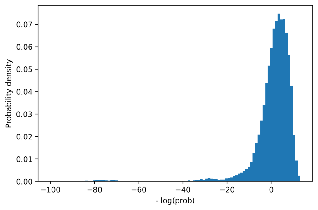
Comparing full joint probabilities

UNCRi’s ability to compute full joint probability density values for any data point enables deeper validation. Histograms of negative log joint probabilities for original and synthetic datasets show similar distributions, further confirming that the synthetic data accurately represents the original statistical structure.

Figure 3: Joint probability density functions for original and synthetic examples.

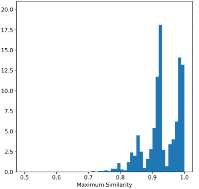
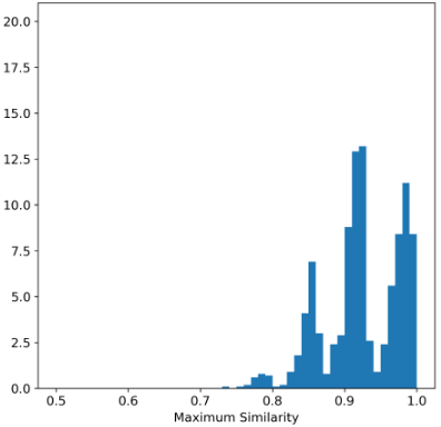
The Maximum Similarity Test

To evaluate privacy and independence of synthetic data, the Maximum Similarity test compares how close synthetic points are to real points relative to real points’ closeness to each other. Ideally, synthetic data should not be closer to real data than real data are among themselves.

Due to dataset size, this test was conducted on random subsets of 1,000 points. The average maximum similarity for original data points (R_max) was 0.932, and between synthetic and original points (S_max) was 0.926, supporting the conclusion that synthetic data is independent and not simply a perturbation of real data.

Histogram comparisons of maximum similarity distributions reinforce this finding.

Figure 4: Histograms of maximum difference between real examples (left), and between synthetic and real examples (right)

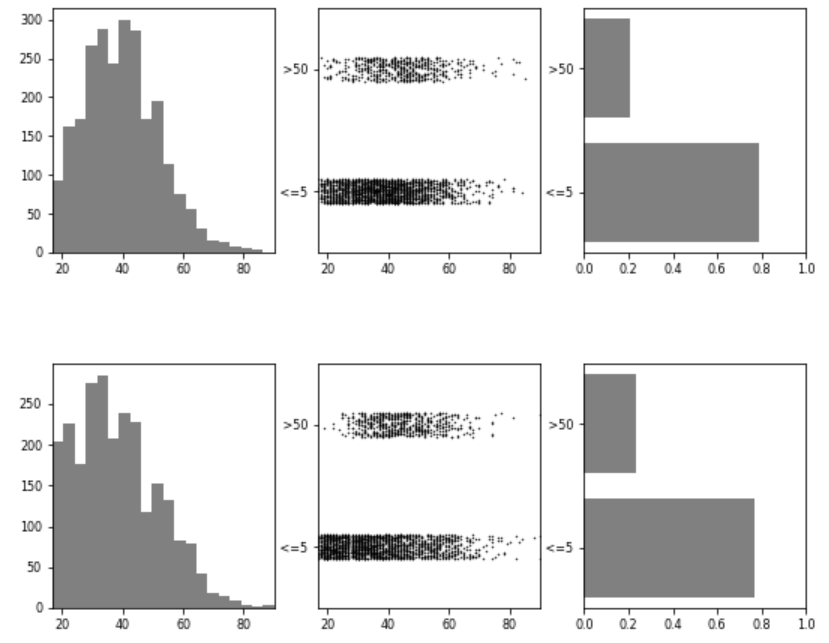
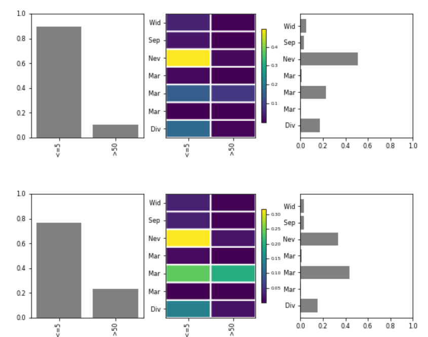
Synthetic Data from Conditional Distributions

UNCRi directly models and samples from conditional distributions, enabling efficient generation of data matching specified attribute conditions. This is more effective than rejection sampling approaches, especially when few original examples meet the condition.

For example, synthetic data conditioned on Race = Amer-Indian-Eskimo and Gender = Female shows distinct distributions for Income and Marital Status when compared to the original data, demonstrating UNCRi’s flexible conditional sampling capability.

The figure below shows the univariate and bivariate distributions for income and marital-status. There are clear differences in the distributions between the generated examples (top) and the original examples (bottom).

Prediction and Imputation

The Income dataset contains missing values. UNCRi’s imputation tool estimates the conditional distribution for missing attributes and assigns random draws from that distribution, preserving data variability. The prediction tool similarly estimates conditional distributions but assigns expected values, useful for filling in missing data with single-point estimates.

Summary

The Income dataset is a standard benchmark for synthetic data evaluation. Our UNCRi model successfully generates synthetic data closely matching original data distributions and preserving predictive relationships, as demonstrated by rigorous validation tests. Privacy-preserving similarity testing confirms that synthetic data is independent from original records. This establishes confidence in UNCRi’s ability to reliably estimate conditional distributions and apply them to a wide range of inference tasks, including data augmentation, classification, and imputation.

Want to know how the Skanalytix Data Generator Stacks up against Competitors

See the following article on Towards Data Science: Evaluating Synthetic Data—The Million Dollar Question